
In this particular section we will talk about ideal transformer and we will also see it’s phasor diagram with proper steps. We have already seen Transformer and it’s working principle.
Definition an properties of ideal transformer
An ideal transformer is an imaginary transformer which has the following properties:
- The resistance of its primary and secondary winding is negligible.
- The permeability (µ) of the core of an ideal transformer is infinite, so that negligible mmf (magnetomotive force) is required to establish the flux in the core.
- The leakage flux and leakage inductances of an Ideal transformer are zero. It means the entire flux is confined to the core and links both windings.
- The losses due to resistance, hysteresis and eddy current are negligible. Hence the efficiency is 100 %.
It should be understood that practical transformer posses none of the above mentioned properties, though the operation of practical transformer is close to ideal one.
Construction of an Ideal transformer
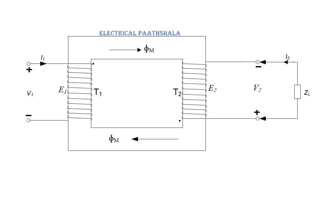
An ideal iron-core transformer is shown in the figure given below. It consists of two coils wound in the same direction on a common magnetic core.
The winding connected to the supply, V1, is called primary and the winding connected to the load, ZL, is called the secondary.
The number of turns in primary and secondary windings are T1 and T2 respectively.
The flux generated \( { \emptyset }_{ m }\) is linked with both the windings as shown in figure below.
Phasor Diagram:
Since, The ideal transformer has zero primary and zero secondary impedance, the voltage induced in the primary E1 is equal to the applied voltage V1.
Similarly, the secondary voltage V2 is equal to the secondary induced voltage E2.
Current I1 is drawn from the supply which is sufficient enough to produce mutual flux ɸM. This current I1 also produce the required magnetomotive force (mmf) I1T1, which is also known as magnetizing mmf , to overcome the demagnetizing effect of the secondary mmf I2T2 as a result of connect load.
Let us take ɸM the reference phasor which is given by
\( \emptyset ={ \emptyset }_{ m }\sin { \omega t } \quad \quad \quad \quad \quad \quad (1) \)EMF E1 and E2 is induced by flux ɸM are given by
\(E_{ 1 }=E_{ 1m }\sin { \left( \omega t-\frac { \pi }{ 2 } \right) } \quad \quad \quad \quad \quad \quad (2)\) \(E_{ 2 }=E_{ 2m }\sin { \left( \omega t-\frac { \pi }{ 2 } \right) } \quad \quad \quad \quad \quad \quad (3)\)
where, E1m and E2m are the maximum value of induced EMF E1 and E2 respectively.
For derivation of Eq.(2) and Eq.(3) click here .
Now, from Eq.(2) and Eq.(3) we can see that, primary induced emf E1 and secondary induced emf E2 lags ɸM by 90o.
By Lenz’s law, E1 is equal and opposite to V1 (i.e. E1 = – V1). Since E1 and E2 both are induced by same mutual flux ɸM. Hence, E1 and E2 both are in same direction and opposite to V1.
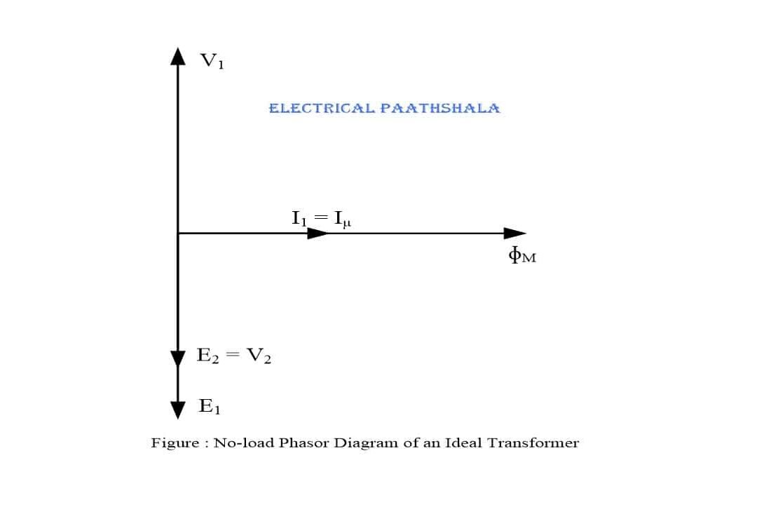
As there is no losses in an ideal transformer, therefore total primary current I1 is used to magnetize the iron-core without any loss due to resistance, hysteresis and eddy currents. So, I1 is equal to the magnetizing current Iµ which lags V1 by 90o and produces mutual flux ɸM in phase with Iµ. V2 is equal in magnitude to E2 and is opposite to V1.
We can relate the above explanation with the help of phasor diagram below,
For an ideal transformer, if
a = transformation ratio = turn ratio
\( then,\quad a=\frac { T_{ 1 } }{ T_{ 2 } } =\frac { E_{ 1 } }{ E_{ 2 } } =\frac { V_{ 1 } }{ V_{ 2 } } =\frac { I_{ 2 } }{ I_{ 1 } } \quad \quad \quad \quad \quad \quad \quad \quad (4) \) \(∴\quad \quad \quad I_{ 1 }T_{ 1 }=I_{ 2 }T_{ 2 }\quad \quad \quad \quad \quad \quad \quad \quad \quad \quad \quad \quad \quad (5)\)Equation (5), states that demagnetizing ampere-turns of the secondary are equal and opposite to the magnetizing mmf of the primary of an ideal transformer.
From equation (4) we get
\(E_{ 1 }I_{ 1 }=E_{ 2 }I_{ 2 }=S_{ 1 }=S_{ 2 }\quad \quad \quad \quad (6)\) \(V_{ 1 }I_{ 1 }=V_{ 2 }I_{ 2 }=S_{ 1 }=S_{ 2 }\quad \quad \quad \quad (7)\)Equation (6), shows that the voltamperes (apparent power) drawn from the primary supply, is equal to the voltamperes (apparent power) transferred to the secondary without any loss, in an ideal transformer. In other words,
Input voltamperes = Output voltamperes
Also, \(\frac { (V_{ 1 }I_{ 1 }) }{ 1000 } =\frac { (V_{ 2 }I_{ 2 }) }{ 1000 } \)
\( { \left( kVA \right) }_{ 1 }\) = \({ \left( kVA \right) }_{ 2 }\) \(\quad \quad \quad \quad \quad \quad (8)\)Input kilovoltamperes = Output kilovoltamperes
From the above discussion, we can say that kVA input of an ideal transformer is equal to the kVA output i.e. kVA is same on both sides of the transformer.
The video for Ideal transformer is here,