
Introduction:
In this blog we will study about “what is transfer function of a control system?” We will talk about the definition of transfer function, types of transfer function, characteristics of transfer function, advantages and disadvantages of transfer function and we will also derive the transfer function of some standard circuits. You will also get to know about poles and zeros of a transfer function and how to draw pole-zero plot for a given transfer function with suitable examples. So, let’s start…
Generally, a physical component is represented by means of a differential equation. A system consists of various physical components, can be represented and described mathematically by a set of differential equations. By using Laplace Transform, these differential equations can be converted into a set of algebraic equations and after that further manipulations can be applied. The most popular and appropriate manipulation is the formulation of Transfer Function. But, what is transfer function?
- The transfer function of a component provides a unique mathematical expression which specifies the characteristics of that component.
- Transfer function is a means of characterizing a system. The complete characterization of a system may require more than one transfer function as there may be multiple inputs and outputs.
- A basic limitation of transfer function is that the system should be linear i.e. it should be represented by a set of differential equations.
- Another limitation is that initial condition of the system should be zero i.e. system should initially be at rest. It means that no energy should be stored in any part of the system initially.
Definition:
The transfer function of a linear, time-invariant (LTI) system is defined as the ratio of the Laplace transform of the output to the Laplace transform of the input under the assumption that all initial conditions are zero.
Transfer function is a rational algebraic function (ratio of two polynomials) in terms of variable ‘s’.
$$T.F.=F\left(s\right)=\left.\frac{L\left({\displaystyle\frac op}\right)}{L\left({\displaystyle\frac ip}\right)}\right|\left(initial\;conditions=0\right)$$
$$T.F.=F\left(s\right)=\frac{C\left(s\right)}{R\left(s\right)}=\left.\frac{Lc\left({\displaystyle t}\right)}{Lr\left({\displaystyle t}\right)}\right|\left(initial\;conditions=0\right)$$
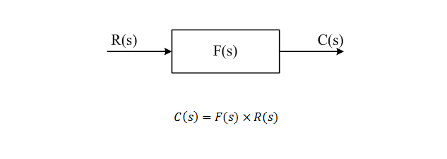
In general, a system with input r(t) and output c(t) can be represented as

$$f\left(t\right)=\frac{c\left(t\right)}{r\left(t\right)}$$
Where, f(t) = System Function
Assuming all the initial conditions to be zero and taking Laplace transform
$$Transfer\;Function=F\left(s\right)=\frac{C\left(s\right)}{R\left(s\right)}=\left.\frac{Lc\left({\displaystyle t}\right)}{Lr\left({\displaystyle t}\right)}\right|\left(initial\;conditions=0\right)$$
A transfer function is that quantity which must be multiplied by the transform of the input for obtaining the transform of the output.
Note:
$$F\left(s\right)=Transfer\;Function$$
$$s=j\omega$$
$$F\left(j\omega\right)=Sinusoidal\;Transfer\;Function$$
What is Linear Time-invariant Systems?
Linear Systems:
The system which follows the “principle of superposition”, are known as Linear Systems.
Liner systems are represented by a set of differential equations.
Principle of Superposition:
Principle of superstition is sufficient and necessary condition to prove the linearity of a system. It means that if a system follows the principle of superposition, then it will surely be a linear system.
Principle of Superposition consists of two laws, which are
- Law of Additivity
- Law of Homogeneity
Law of Additivity
Law of additivity states that if the response of a given system is y1(t) for input x1(t) and y2(t) for input x2(t), then for the sum of input [x1(t) + x2(t)], the response of the system will be [y1(t) + y2(t)].
$$if\;f\left\{x_1\left(t\right)\right\}=y_1\left(t\right)$$
$$and\;f\left\{x_2\left(t\right)\right\}=y_2\left(t\right)$$
$$then,\;f\left\{x_1\left(t\right)+x_2\left(t\right)\right\}=y_1\left(t\right)+y_2\left(t\right)$$

In other words, we can say that, for a given system the net response caused by two or more input is the sum of the responses that would have been caused by each input individually.
The general definition can be given as, when multiple inputs x1(t), x2(t),….., xn(t) acts simultaneously on a given system then the net response y(t) is equals to the sum of responses of each individual input under the assumption that all initial conditions of the system are zero.
Therefore, if yi(t) is the response of the system for input xi(t), then the relationship given below holds true:
$$y\left(t\right)=\sum_{i=1}^ny_i\left(t\right)$$
Law of Homogeneity
Law of homogeneity states that, if the input of the system x(t) is multiplied by a constant K then the output of the system y(t) will also be multiplied by the same constant K.
$$if\;f\left\{x\left(t\right)\right\}=y\left(t\right)$$
$$then,\;f\left\{Kx\left(t\right)\right\}=Kf\left\{x\left(t\right)\right\}=Ky\left(t\right)$$
Where K is a constant.
In other words, we can say that if input of the system is scaled by a constant then the same scaling factor will be reflected in the output also.

So, if a system follows both Law of Additivity and Law of Homogeneity then we can say that the system follows the Principle of Superposition and it’s a Linear System. But if the system violates even one of these laws, then the system does not follow Principle of Superposition and it is said to be a Non – Linear System.
Time-Invariant System:
The system for which output of the system does not depend on the time of application of input are known as Time – Invariant Systems.
For time – invariant systems, if there is some delay in the input, it must be reflected in the output also i.e. if the input is delayed by t0then the output must also be delayed by time t0.

Those systems which are linear as well as time – invariant, are called as Linear Time – Invariant (LTI) Systems.
LTI systems are represented by constant coefficient differential equations.
Why initials conditions are assumed to be zero to write Transfer Function?
There is a property of linear systems that for zero input, the output of the system must be zero.

Now, a system gives output in two conditions
- Some input is applied.
- There are some initial conditions.
Suppose, applied input is zero but there are some initial conditions. In this case even if the input is zero, the system will give some output because of initial conditions. But this will violate the property of linear systems. That’s why, to write transfer function, initial conditions of the system are assumed to be zero.
Transfer Function of Some Standard Circuits
Series RC Circuit

Applying KVL
$$V_i\left(t\right)=i\left(t\right)R+\frac1C\int i\left(t\right)\cdot dt$$
$$V_0\left(t\right)=\frac1C\int i\left(t\right)\cdot dt$$
Taking Laplace Transform
$$V_i\left(s\right)=I\left(s\right)R+\frac1{sC}I\left(s\right)$$
$$\Rightarrow V_i\left(s\right)=\left[R+\frac1{sC}\right]I\left(s\right)$$
and $$V_0\left(s\right)=\frac1{sC}I\left(s\right)$$
For obtaining transfer function
$$Transfer\;Function=\frac{Laplace\;of\;Output}{Laplace\;of\;Input}=\frac{V_0\left(s\right)}{V_i\left(s\right)}$$
$$T.F.=\frac{\displaystyle\frac1{sC}}{R+{\displaystyle\frac1{sC}}}=\frac1{1+sRC}$$
$$T.F.=F\left(s\right)=\frac1{1+\tau s}$$
$$Here,\;\tau=RC=Time\;Cons\tan t\;of\;Series\;RC\;Circuit$$
Series RL Circuit

Applying KVL
$$V_i\left(t\right)=i\left(t\right)R+L\frac{di\left(t\right)}{dt}$$
$$V_0\left(t\right)=L\frac{di\left(t\right)}{dt}$$
Taking Laplace Transform
$$V_i\left(s\right)=I\left(s\right)R+sLI\left(s\right)$$
$$and\;V_0\left(s\right)=sLI\left(s\right)$$
For obtaining transfer function
$$Transfer\;Function=\frac{Laplace\;of\;Output}{Laplace\;of\;Input}=\frac{V_0\left(s\right)}{V_i\left(s\right)}$$
$$T.F.=\frac{sLI\left(s\right)}{I\left(s\right)\left(R+sL\right)}=\frac{sL}{R+sL}=\frac{s\left({\displaystyle\frac LR}\right)}{1+s\left({\displaystyle\frac LR}\right)}$$
$$T.F.=F\left(s\right)=\frac{\tau s}{1+\tau s}$$
$$Here,\;\tau=\frac LR=Time\;Cons\tan t\;of\;Series\;RL\;Circuit$$
Series RLC Circuit

Applying KVL
$$V_i\left(t\right)=i\left(t\right)R+L\frac{di\left(t\right)}{dt}+\frac1C\int i\left(t\right)\cdot dt$$
$$V_0\left(t\right)=\frac1C\int i\left(t\right)\cdot dt$$
Taking Laplace Transform
$$V_i\left(s\right)=I\left(s\right)R+sLI\left(s\right)+\frac1{sC}I\left(s\right)$$
$$\Rightarrow V_i\left(s\right)=\left[R+sL+\frac1{sC}\right]I\left(s\right)$$
$$and,\;V_0\left(s\right)=\frac1{sC}I\left(s\right)$$
For obtaining transfer function
$$Transfer\;Function=\frac{Laplace\;of\;Output}{Laplace\;of\;Input}=\frac{V_0\left(s\right)}{V_i\left(s\right)}$$
$$T.F.=\frac{\displaystyle\frac1{sC}}{R+sL+{\displaystyle\frac1{sC}}}=\frac1{LCs^2+RCs+1}$$
CLOSE LOOP TRANSFER FUNCTION

$$C\left(s\right)=G\left(s\right)\cdot E\left(s\right)\;\;\;\;….\left(1\right)$$
$$B\left(s\right)=H\left(s\right)\cdot C\left(s\right)\;\;\;\;….\left(2\right)$$
$$E\left(s\right)=R\left(s\right)-C\left(s\right)$$
Using eq.(1) and eq.(2)
$$\frac{C\left(s\right)}{G\left(s\right)}=R\left(s\right)-H\left(s\right)\cdot C\left(s\right)$$
$$\Rightarrow C\left(s\right)=G\left(s\right)R\left(s\right)-G\left(s\right)H\left(s\right)C\left(s\right)$$
$$\Rightarrow C\left(s\right)+G\left(s\right)H\left(s\right)C\left(s\right)=G\left(s\right)R\left(s\right)$$
$$\Rightarrow\left[1+G\left(s\right)H\left(s\right)\right]C\left(s\right)=G\left(s\right)R\left(s\right)$$
$$\Rightarrow\frac{C\left(s\right)}{R\left(s\right)}=\frac{G\left(s\right)}{1+G\left(s\right)H\left(s\right)}$$
The above expression is called as Close Loop Transfer Function (C.L.F.T.).

OPEN LOOP TRANSFER FUNCTION
$$\frac{C\left(s\right)}{R\left(s\right)}=G\left(s\right)=O.L.T.F.$$
The above expression is called as Open Loop Transfer Function (O.L.F.T.).

Shortcut Method:
Suppose, Given
$$C.L.T.F.=\frac{Num}{Den}$$
Then,
$$O.L.T.F.=\frac{Num}{Den-Num}$$
TYPES OF TRANSFER FUNCTION
Suppose a transfer function is given by
$$T.F.=F\left(s\right)=\frac{C\left(s\right)}{R\left(s\right)}=\frac{b_0s^m+b_1s^{m-1}+…..+b_m}{a_0s^n+a_1s^{n-1}+…..+a_n}$$
Case-1:
If (Degree of denominator Polynomial) > (Degree of numerator Polynomial)
i.e n > m
Then this type of transfer function is known as Strictly Proper.
Case-2:
If (Degree of denominator Polynomial) = (Degree of numerator Polynomial)
i.e n = m
Then this type of transfer function is known as Proper.
Case-3:
If (Degree of denominator Polynomial) < (Degree of numerator Polynomial)
i.e n < m
Then this type of transfer function is known as Improper.
POLES AND ZERO
Suppose a transfer function is given by
$$T.F.=F\left(s\right)=\frac{C\left(s\right)}{R\left(s\right)}=\frac{b_0s^m+b_1s^{m-1}+…..+b_m}{a_0s^n+a_1s^{n-1}+…..+a_n}$$
Factorizing numerator and denominator polynomials
$$T.F.=F\left(s\right)=\frac{C\left(s\right)}{R\left(s\right)}=\frac{K\left(s-z_1\right)\left(s-z_2\right)…….\left(s-z_m\right)}{\left(s-p_1\right)\left(s-p_2\right)…….\left(s-p_n\right)}$$
Here, K = System Gain or Gain Factor
Definition of Poles:
$$For\;s=p_1,p_2,…….p_n$$
Magnitude of transfer function
$$\left|T.F.\right|=\left|F\left(s\right)\right|=\infty$$
Those critical frequencies for which magnitude of transfer function becomes infinite, are known as the Poles of the system.
- If poles are not repeated then they are called as Simple Poles.
- If poles are repeated (more than one pole at one location) then they are called as Multiple Poles.
Definition of Zeros:
$$For\;s=z_1,z_2,…….z_m$$
Magnitude of transfer function
$$\left|T.F.\right|=\left|F\left(s\right)\right|=0$$
Those critical frequencies for which magnitude of transfer function becomes zero, are known as the Zeros of the system.
- If zeros are not repeated (only one zero at one location) then they are called as Simple Zeros.
- If zeros are repeated (more than one zero at one location) then they are called as Multiple Zeros.
Example: Given,
$$T\left(s\right)=\frac{s^2+6s+9}{s^3+s^2+14s+8}$$
Factorizing Numerator & Denominator Polynomials
$$T\left(s\right)=\frac{\left(s+3\right)^2}{\left(s+1\right)\left(s+2\right)\left(s+4\right)}$$
Conclusions:
- There are two zeros at s = -3
Therefore, (s+3) is a multiple zero with multiplicity 2.
- There are three poles of the system which are at s = -1, s = -2, s = -4
(s+1), (s+2) and (s+4) are simple poles.
Poles & Zeros at Infinite
Suppose, transfer function of a system is given by
$$T.F.=F\left(s\right)=\frac{C\left(s\right)}{R\left(s\right)}=\frac{b_0s^m+b_1s^{m-1}+…..+b_m}{a_0s^n+a_1s^{n-1}+…..+a_n}$$
Case-1:
$$if,\;m>n,\;then$$
$$For\;s=\infty$$
$$\left|T.F.\right|=\left|F\left(s\right)\right|=\infty$$
$$There\;exists\;a\;pole\;at\;s=\infty$$
Case-2:
$$if,\;m<n,\;then$$
$$For\;s=\infty$$
$$\left|T.F.\right|=\left|F\left(s\right)\right|=0$$
$$There\;exists\;a\;zero\;at\;s=\infty$$
Conclusion: For a rational transfer function, number of poles is always equals to number of zeros.
Number of Poles = Number of Zeros
Pole – Zero Plot
Pole – zero plot means representation of poles and zeros in s-plane.
Here, s-plane = space plane
$$s=\sigma+j\omega$$
Where, σ = Real Values = Values on Real Axis
ω = Imaginary Values = Values on Imaginary Axis
$$s=\lim_{R\rightarrow\infty}\left(Re^{j\theta}\right)$$

In s-plane, poles are denoted by cross (x) and zeros are denoted by a small circle or dot (o).
If there are more than one pole or zero at one location (multiple poles or multiple zeros) then it is representation by overlapped cross or overlapped dot respectively.
Example:
$$T\left(s\right)=\frac{\left(s+3\right)^2}{\left(s+1\right)\left(s+2\right)\left(s+4\right)}$$
The pole-zero plot of the given transfer function is shown in the figure below:

*Three Simple Poles At
s = -1, s = -2 and s = -4
*Two Multiple Zeros At
s = -3
Time Constant Form of Transfer Function
$$T.F.=F\left(s\right)=\frac{K\left(s+z_1\right)\left(s+z_2\right)}{\left(s+p_1\right)\left(s+p_2\right)}$$
The above expression is known as the General Form of transfer function.
$$\Rightarrow T.F.=F\left(s\right)=\frac{Kz_1\left(1+{\displaystyle\frac s{z_1}}\right)z_2\left(1+{\displaystyle\frac s{z_2}}\right)}{p_1\left(1+{\displaystyle\frac s{p_1}}\right)p_2\left(1+{\displaystyle\frac s{p_2}}\right)}$$
$$\Rightarrow T.F.=F\left(s\right)=\frac{Kz_1z_2\left(1+{\displaystyle\frac s{z_1}}\right)\left(1+{\displaystyle\frac s{z_2}}\right)}{p_1p_2\left(1+{\displaystyle\frac s{p_1}}\right)\left(1+{\displaystyle\frac s{p_2}}\right)}$$
$$\Rightarrow T.F.=F\left(s\right)=\frac{K^{‘}\left(1+T_as\right)\left(1+T_bs\right)}{\left(1+T_1s\right)\left(1+T_2s\right)}$$
The above expression is known as the Time – Constant Form of transfer function.
Here,
$$K^{‘}=\frac{Kz_1z_2}{p_1p_2}=D.C.\;Gain\;of\;The\;System$$
And Ta = 1/z1, Tb = 1/z2, T1 = 1/p1, T2 = 1/p2 are called as Time Constants.
Characteristics Polynomial:
The denominator polynomial in variable ‘s’ of the transfer function is called as Characteristic Polynomial.
Characteristics Equation:
The denominator polynomial in variable ‘s’ of the transfer function when equated to zero, is called as Characteristic Equation of that transfer function.
Example:
$$T\left(s\right)=\frac{s^2+6s+9}{s^3+s^2+14s+8}$$
Characteristic Polynomial
$$s^3+s^2+14s+8$$
Characteristic Equation
$$s^3+s^2+14s+8=0$$
PROPERTIES OF TRANSFER FUNCTION
1. The transfer function can be determined from system input – output just by taking ratio of Laplace transform of output tom Laplace transform of input.
2. System differential equation can be obtained from transfer function by replacing ‘s’ variable with linear differential operator ‘D’.
$$Here,\;D\equiv\frac d{dt}$$
This means that it is an operational method of expressing differential equation that relates the output variable to the input variable.
Consider a system with input r(t) and output c(t) which is represented by differential equation
$$a_0\frac{d^2c\left(t\right)}{dt^2}+a_1\frac{dc\left(t\right)}{dt}+a_2c\left(t\right)=b_0\frac{d^2r\left(t\right)}{dt^2}+b_1\frac{dr\left(t\right)}{dt}+b_2r\left(t\right)$$
Where a0, a1, a2, b0, b1, b2 are constants.
Assuming initial conditions to be zero and taking Laplace transform, we will obtain
$$a_0s^2C\left(s\right)+a_1sC\left(s\right)+a_2C\left(s\right)=b_0s^2R\left(s\right)+b_1sR\left(s\right)+b_2R\left(s\right)$$
$$\Rightarrow\left[a_0s^2+a_1s+a_2\right]C\left(s\right)=\left[b_0s^2+b_1s+b_2\right]R\left(s\right)$$
$$\Rightarrow\frac{C\left(s\right)}{R\left(s\right)}=\frac{b_0s^2+b_1s+b_2}{a_0s^2+a_1s+a_2}$$
3. Transfer function is defined only for linear time – invariant systems. It is not defined for non – linear or time variant systems.
4. To write transfer function of a system all initial conditions are assumed to be zero.
5. System poles and zeros can be found out by using transfer function.
6. The stability of the system can be determined from its characteristics equation if transfer function is given.
7. Transfer function is a property of the system and it is independent of the magnitude and nature of the input applied.
8. Transfer function can be used to find the output of the system if input is known and vice – versa.
Advantages of Transfer Function
1. Transfer function gives simple mathematical algebraic equation.
2. Gain can easily be determined for a system whose input and output is given.
3. Transfer function gives poles and zeros of the system directly.
4. Stability of the system can be determined easily by using transfer function.
5. The output of the system for any input can be determined easily if transfer function is given.
Disadvantages of Transfer Function
1. Transfer function is valid only for linear time – invariant (LTI) systems.
2. It does not take initial conditions of the system into account.
3. It does not mention anything about the internal state of a system.
4. Analysis of multiple input – multiple output (MIMO) is cumbersome by using transfer function.
5. Controllability and Observability cannot be determined by using transfer function.
Watch What is Transfer Function?
Read More: